Microeconomic and Macroeconomic Perspectives on Public Policy

1.

In a private market for higher education, the supply and demand for education are determined by individuals and institutions without government intervention. The equilibrium in such a market is where the quantity of schooling supplied matches the quantity demanded at a specific price, as shown in Figure 1 below.

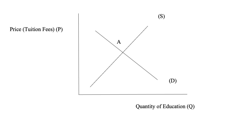
The horizontal axis symbolizes the quantity of education, and the vertical axis signifies the price (tuition fees). Market equilibrium is at place A, where private education (Q) is supplied at the confidential market price (P). The level of education may not be socially optimal due to market failures such as:

Positive Externalities: Education makes positive externalities, showing that the importance of education extends beyond the discrete learner to society as a whole. External benefits include an extra knowledgeable and skilled workforce, reduced crime charges, progressed fitness results, and improved innovation, not pondered inside the private marketplace equilibrium.

Underinvestment: In a private market, individuals consider only their benefits when deciding how much education to pursue. They do not take into account the positive externalities. As a result, the private market will tend to underprovide education, stopping short of the socially optimal level (Q in Figure).

b) Socially Optimal Level with Government Funding:

When the government intervenes to fund higher education, it can correct the market failure by providing subsidies or funding to increase the quantity of education to the socially optimal level, as shown in Figure 2 below.

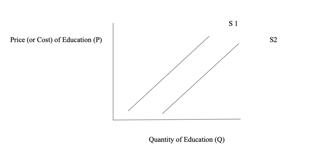
Government subsidy makes the curve move to the right, increasing the quantity of education to Q. It covers part of the cost, reducing the price students pay to P. As a result, more students can afford higher education, leading to higher enrollment in STEM disciplines and other areas supported by the government.

Comparing this outcome to the previous equilibrium (point A), it is evident that government funding boosts the quantity of education to the socially optimal level (Q), where the positive externalities are considered. It ensures society benefits from a more educated workforce, technological advancements, and other positive spillover effects that private markets alone cannot achieve.

2.

Between July 2021 and July 2023, the trend in gross domestic consumer expenditure can be expected to reflect the broader economic conditions during this period, particularly the impact of rising inflation and its effect on consumers' confidence. Increasing inflation tends to erode the purchasing power of consumers, leading to changes in their spending behavior (Bennett, 2020). As inflation persists and deteriorates their actual income, they may cut back on discretionary spending, leading to a slowdown in consumer expenditure, though consumers might continue spending.

In the Keynesian Cross model, changes in consumer expenditure play a crucial role in determining the equilibrium output. The model suggests that total spending in an economy (aggregate demand) determines economic output (GDP). Consumer expenditure is a significant component of aggregate demand. Once consumers are confident and have strong purchasing power, they tend to spend more, increasing aggregate demand. While they become less optimistic due to rising inflation and stagnant wages, they may reduce their spending, causing a decrease in aggregate demand.

As consumer expenditure declines, the equilibrium output in the Keynesian Cross model also decreases. It is because the total spending in the economy falls, reducing production and, consequently, GDP. In the context of the alleged impact of weaker consumer confidence due to rising inflation on slower economic growth between July 2021 and July 2023, it can be expected that a decline in consumer expenditure during this period would contribute to a lower equilibrium output. A slowdown in economic activity necessitates policy measures to stimulate consumer spending and boost demand to support economic growth.

3.

As of the latest available data in August 2023, the unemployment rate in Australia stands at 3.7%. The natural unemployment rate is the unemployment level in an economy when it operates at its potential or total employment output. It includes frictional and structural unemployment but excludes cyclical unemployment (Bennett, 2020). The economic system is operating at complete employment if the unemployment rate is identical to or very close to the herbal price. In instances where the actual unemployment fee is higher than the delivery rate, it shows the presence of cyclical unemployment. It suggests that the economy is not at complete employment.

Discouraged unemployment refers to individuals who have given up attempting to find employment because they believe that no suitable employment opportunities are available. Persons are not counted in the legitimate unemployment rate because they are not actively seeking employment. The natural unemployment price does not include discouraged unemployment; the modern published unemployment price, which is 3.7% in August 2023, represents the cyclical unemployment rate, the portion of unemployment resulting from fluctuations within the commercial enterprise cycle. It is the difference between the actual and natural rate of unemployment (NAB Group Economics, 2023). The unemployment rate is lower than the birth rate, indicating that the economy is experiencing cyclical idleness and is not operating at full employment.

Causes of Cyclical Unemployment:

It is primarily caused by economic recessions or downturns when overall economic activity declines. During these periods, businesses may reduce production, leading to layoffs and decreased labor demand. When consumer spending decreases due to economic uncertainty, businesses may scale back operations and hire fewer workers, contributing to cyclical unemployment. A decrease in business investment, often driven by reduced confidence in the economy, can lead to reduced job creation and cyclical unemployment.

Consequences of Cyclical Unemployment:

Workers who become unemployed during economic downturns may face income loss, resulting in financial hardship for individuals and families. Cyclical unemployment reduces production and output as fewer workers contribute to economic activity. High levels of cyclical unemployment can further dampen consumer spending, leading to a prolonged economic downturn.

4.

a) The aggregate expenditure function in this economy can be calculated as follows:

AE=C+I+G+ (X−M)

Where:

C is consumption expenditure, given as =100+0.8 C=100+0.8YD.

I am a planned investment, given as =40I=40.

G is government expenditure, given as =50G=50.

X is exported, given as =20X=20.

M is imported, given as =10+0.06 M=10+0.06Y.

Y equals aggregate expenditure (AE).

AE = (100+0.8)+40+50+(20−(10+0.06))AE=(100+0.8YD)+40+50+(20−(10+0.06Y)) =190+0.8−0.06AE=190+0.8YD−0.06Y

Disposable income (YD) equals real GDP (Y).

=190+0.8−0.06AE=190+0.8Y−0.06Y =190+0.74 AE=190+0.74Y

Now, we set AE equal to Y to find the equilibrium level of income:

AE=Y 190+0.74=190+0.74Y=Y

Solving for Y:

0.74=1900.74Y=190 =1900.74=256.76Y=0.74190​=256.76

The equilibrium level of income in the economy is approximately $256.76 billion.

b)

To find the value of consumption expenditure (C) for the economy, we can use the consumption function given:

100+0.8C=100+0.8YD

Since YD is equal to Y in this case (as mentioned earlier), we have:

=100+0.8C=100+0.8Y

Now, plug in the equilibrium level of income (Y) calculated in part (a):

=100+0.8×256.76C=100+0.8×256.76 =307.41C=307.41

The value of consumption expenditure for the economy is approximately $307.41 billion.

c)

Multiplier=1−MPC1​

MPC=ΔYΔC​

Given that government expenditure falls from $50 billion to $40 billion, the change in government spending (ΔG) is:

=40−50=−10ΔG=40−50=−10

ΔC=Multiplier×ΔG

We know that Multiplier = 11−1−MPC1, so we need to find MPC first. Using the consumption function:

=100+0.8 C=100+0.8Y

We can find MPC as follows:

=0.8MPC=dYdC​=0.8

Now, we can calculate the multiplier:

=11−0.8=10.2=5Multiplier=1−0.81​=0.21​=5

Now, calculate ΔC:

Δ=5× (−10) =−50ΔC=5× (−10) =−50

So, the change in consumption expenditure is $ 50 billion. This means that when government expenditure falls by $10 billion, consumption expenditure decreases by $50 billion.